Request a Dayshape demo
Get in touch and learn first-hand how Dayshape can help boost profitability, improve client service, and keep your teams happy.
Platform
Strategic resource management
Optimize margins. Grow revenue.
Plan reliably. Act confidently.
Inspire teams. Delight clients.
Enterprise scalability
Use Cases
How Dayshape helps firms
10 ways for resource managers to elevate their impact

Elevate your role, expand your influence, and drive impact across your firm.
Listen nowCustomer Success
Value at every stage
Company
More about Dayshape
Resources
Learn more
Resources
Featured resources
Resource Management Maturity

The complete blueprint to transform your resource management.
Learn moreI have always liked the pithy Pablo Picasso quote “[Computers] are useless. They can only give you answers”. But what he may have overlooked is that getting computers to give you decent answers is not a trivial task.
One of the initial instigators to start Dayshape was that I enjoyed solving decision problems. For me, it is something that sits apart from just general programming and I think there’s a concise beauty to a good optimisation model. Hopefully, this article should give you a flavour of that. Perhaps even Pablo could appreciate it!
Dr Alastair Andrew, CTO & Co-Founder of Dayshape
***
Alex Bellos’s bi-weekly column in The Guardian is a good source of diversion to exercise your grey matter on a Monday. Many of the problems also serve as nice examples that you can practice modelling as decision problems.
We’ll look at how to do this for one puzzle, “A Study in Eggs” from the Easter Monday edition.
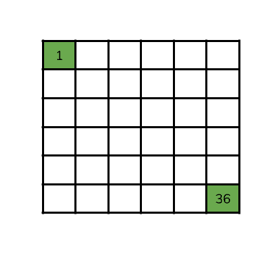
It asks “How many eggs can you place in a 6 by 6 crate such that no row, column, or diagonal has more than 2 eggs in it?” The accompanying diagram shows that two eggs have already been placed in the crate at opposite corners.
One of the regular tropes in the Dayshape office is the Phil Karlton quote “There are only two hard things in Computer Science: cache invalidation and naming things.” I would add the corollary: sometimes the hard thing is knowing what existing things are called.
On its surface “The Study in Eggs” puzzle appears similar to the Eight Queens problem. The eight queens problem asks “Can 8 queens be placed on a regular 8 by 8 chessboard such that no queen can attack another?” The n-queens generalisation, where the chessboard can be increased to any size, is frequently used to demonstrate the concise modelling of Constraint Satisfaction Problems.
Are the two puzzles the same? Let’s start by comparing the setup.
The eggs problem is a 6 by 6 grid; this would be equivalent to an n-queens chessboard where n is 6. In chess, queens can move any number of spaces on a row, column, or diagonal. Again similar.
However, the stipulation that no queen can attack another means we can have at most one queen in each dimension (unlike in the eggs puzzle which allows at most two eggs per dimension).
The final distinction is the actual question. For the n-queens problem, we know the number of queens and the question is to find a valid placement (if this is possible). For the eggs problem, we know the size of the grid but we want to know the largest number of eggs that can be placed whilst respecting the rules. The n-queens problem is a Constraint Satisfaction Problem whereas the eggs problem is a Constraint Optimisation Problem.
To formulate any flavour of constraint problem we need to define our variables; these are decisions we need to make.
In the eggs problem we know we’ve got 36 (i.e. 6 * 6) positions in the crate and we need to decide whether that space should contain an egg or not.
We’ll use the MiniZinc modelling language to express this more formally.
array[1..36] of var 0..1: eggs;
Here we’ve said we’ve got an array called eggs which consists of 36 variables and those variables need to be either 0 or 1 (the variable’s domain). This is the common way of modelling boolean choices used in both Constraint Programming and Integer Programming. Zero represents no egg and one (unsurprisingly) one egg. Our choice of domain prevents us from ever considering more than one egg in any space.
We then need to state the objective. We want to count the number of eggs in the crate.
<sup><kbd>count(e in 1..36)(eggs[e] = 1)</kbd></sup>
This is a function that iterates across the array and returns the number of elements that satisfy the second part. This will look slightly strange to programmers who usually expect a single equals to denote assignment, not an equality comparison.
Next, we need to convey that we want to use this as our objective:
solve maximize count(e in 1..36)(eggs[e] = 1);
The final thing we need to form a valid MiniZinc model is an output statement to print the solution we find.
output [ show2d(array2d(1..6, 1..6, eggs)) ]
To get a nice visual representation of the egg crate it would be better to have a 2d array rather than a flat 1d array. The inner function, array2d, takes our single array and reshapes it into a multidimensional array with the number of rows and columns specified. The show2d function puts in new lines so it’ll print this array nicely.
We can run our model from the command line like so:
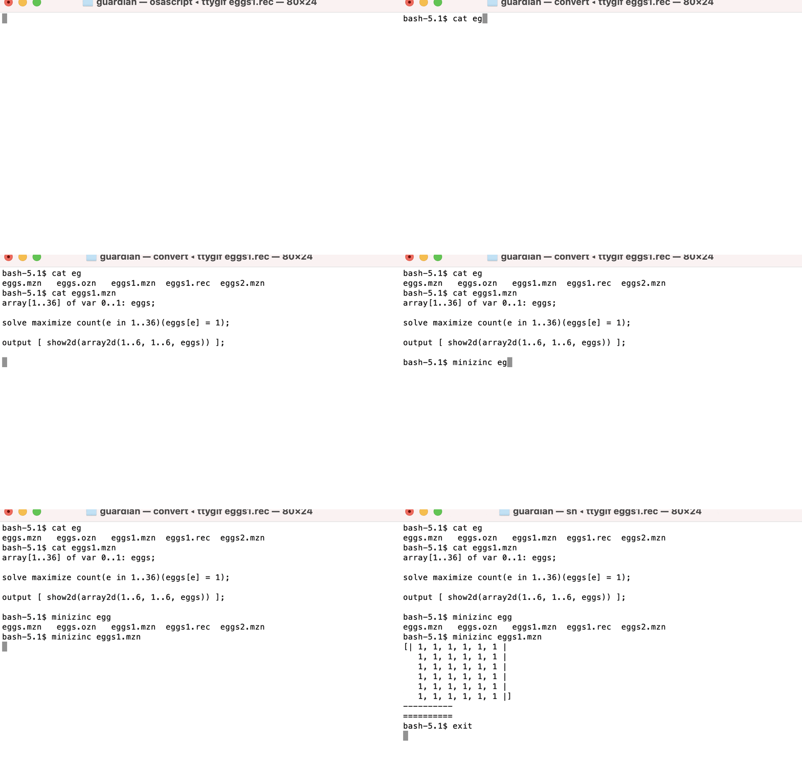
If we solve this model we get a full grid of 36 eggs. We haven’t included any of the rules of the problem in our model yet, so 36 is the maximum number of eggs we could ever fit in the crate.
The restrictions on what is allowed in a valid solution are called constraints. Constraints in a MiniZinc model are prefaced with the keyword constraint.
The simplest two constraints are fixing the existing values:
constraint eggs[1] = 1;
constraint eggs[36] = 1;
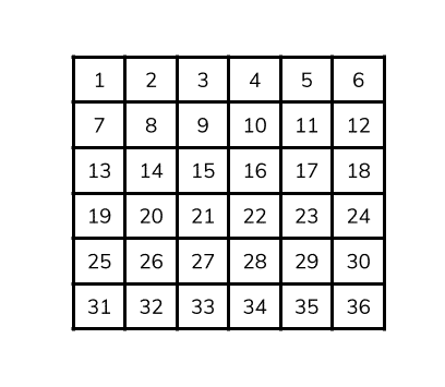
In our model, the eggs array the spaces are numbered 1 to 36 and correspond to the grid starting at the top-left corner and finishing at the bottom right.
Next, we need to enforce the main restriction, no more than 2 eggs on any particular row, column, or diagonal. We’ve seen the count construct used as part of our objective. We can use this as part of our constraints. The count returns the number of matches as an integer and we can use that as the left-hand side of a less-than-or-equal-to constraint.
For the row constraints we could state them as:
constraint count(e in 1..6)(eggs[e] = 1) <= 2;
constraint count(e in 7..12)(eggs[e] = 1) <= 2;
Etc.
Rather than expressing each row explicitly, we can use the forall construct. It works like a loop creating the constraints contained within and stating they all must be satisfied. The only complication is getting our indices correct.
We’ve already seen the array2d function which allows us to reshape an array into a matrix (of the same variables). We can use this to get our variables into a form that makes stating the constraints we need much simpler.
array[1..6,1..6] of var 0..1: crate = array2d(1..6,1..6, eggs);
Now defining the row and column constraints becomes easy to read:
constraint forall(r in 1..6)(count(c in 1..6)(crate[r,c] = 1) <= 2);
constraint forall(c in 1..6)(count(r in 1..6)(crate[r,c] = 1) <= 2);
Notice we’ve kept the matrix indexing as row, column, but flipped the generators between the two versions; one covering the rows, the other constraining the columns.
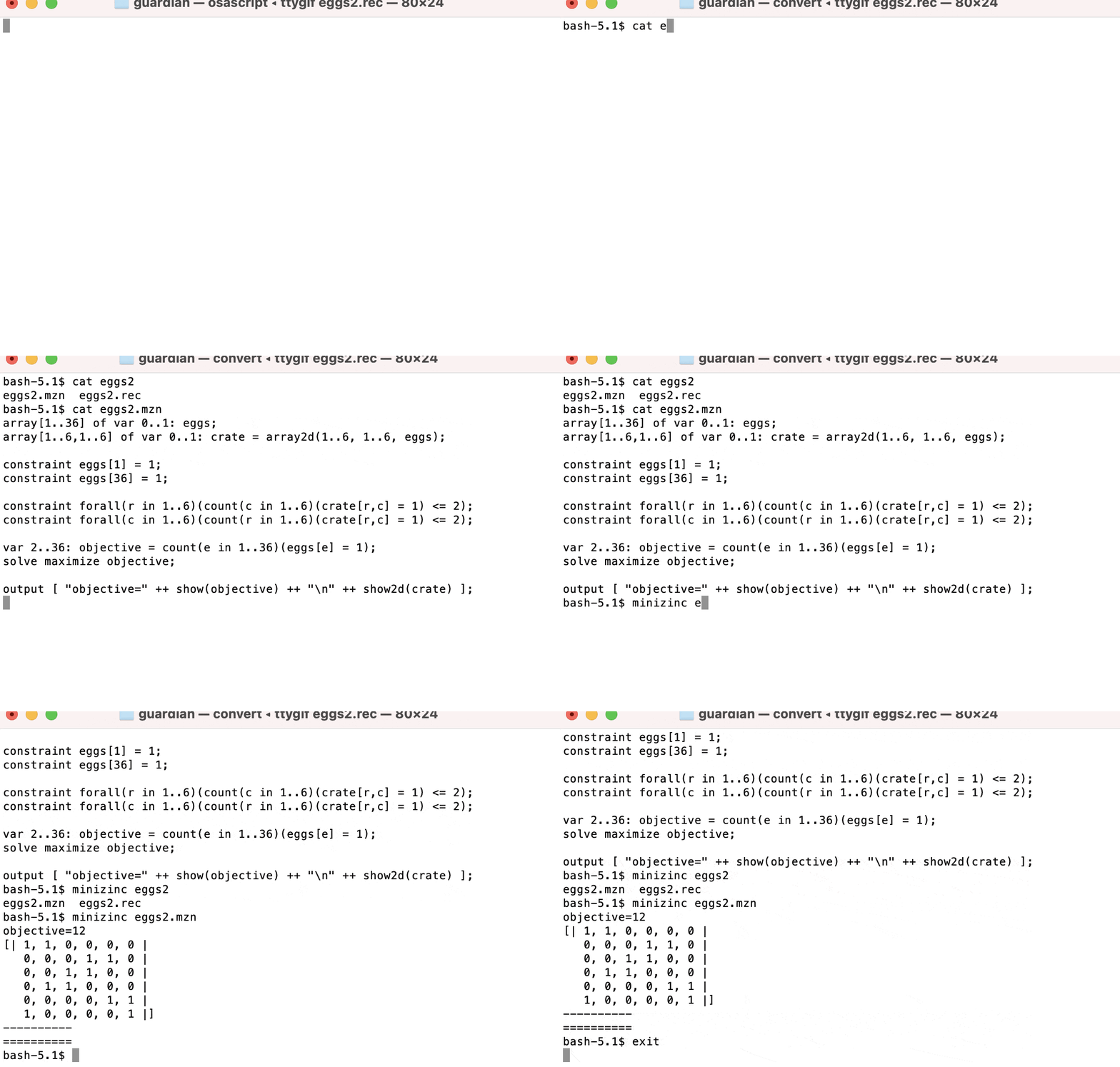
If we run our model now we’ll find that the maximum number of eggs we can place is 12. Intuitively this makes sense; if we’ve got 6 rows and we know we can have a maximum of 2 eggs on that row then we can never place more than 12 eggs on a 6 by 6 grid. This gives an upper bound to our objective.
However, we also know we’ve got extra constraints to add to our model and those constraints can only remove potentially valid positions not add any. So the question is: will 12 be the maximum, or is it actually less?
We still need to add the diagonal restrictions. We know we’ll need to use the count constraint; this time collecting the cells which form a diagonal is not as easy as the rows or columns. For starters, the number of elements in a diagonal slice varies with only the main corner-to-corner diagonal having the maximum 6 elements.
It’s useful to visualise the grid with the positions, this will help us figure out which cells we need to include in each constraint. We know we’ll need to create one counting constraint per diagonal so first we’ll need to work out how many of those there’ll be.
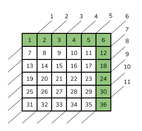
As we can see it’s 11 (i.e. (n * 2) - 1).
The next thing we need to work out is for each of these diagonals, how many squares will be in it?
If we look we can see it’ll be 1, 2, 3, 4, 5, 6, 5, 4, 3, 2, 1. We can generate this using this formula:
array[1..11] of int: lengths = [ 6 - abs(6 - k) | k in 1..11 ];
We could omit the diagonals with only a single element as we know the 0-1 domain of those cells will prevent them from ever violating the count constraint.
So we know the number of loops in our forall statement and we know for each one of those how many elements we expect our count constraint to need. How do we select the right indices? Well for the rows and columns, each loop starts on the lowest position element and iterates for the number of elements in that row/column, collecting the remaining cells.
If we start at the first cell and consider the forward diagonals then we can see from the diagram that the start positions would be: 1,2,3,4,5,6,12,18,24,30,36.
We could fix these start indices in our model like so:
array[1..11] of int: starts = [ 1,2,3,4,5,6,12,18,24,30,36];
Alternatively, we could collect these by using an array comprehension with a where clause. The advantage of defining the comprehension is we’ll be able to more easily abstract our model to ultimately operate over any sized problem.
array[1..11] of int: starts [ i | i in 1..36 where i <= 6 \/ i mod 6 = 0]
In MiniZinc an or operator is \/ using the disjunction notation (rather than the || programmers tend to expect). The mod operator is the modulo. This is just the remainder from a division. So we’re saying either the value is 6 or less, or it can be divided by 6 exactly.
So we’ve got our number of constraints, the starting element for each diagonal and number of elements in each diagonal constraint. How do we figure out the remaining elements? Again if we refer to our diagram it should be possible to discern the pattern.
Ignoring the first diagonal (since it has only one element) and looking at the second and third we see they contain cells 2, 7, and 3, 8, 13 respectively. For the forward diagonals, all the elements are 5 positions apart.
Putting it all together we can create the constraints like:
constraint forall(d in 1..11) count(i in 0..lengths[d] - 1)(eggs[start[d] + (i * 5)] = 1) <= 2;
The same process lets us work out the opposite set of diagonals. We know there’s the same number and each one will be the same length.
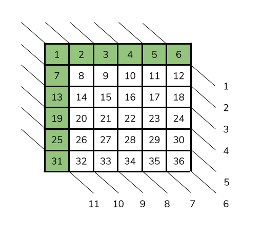
What changes are the starting elements and the pattern of the differences? Referring to the diagram we can see they differ by 7 this time. Why 5 and 7? Well, they are really 6 +/- 1.
Okay, so our model is complete, we’ve expressed all the constraints. What do we get?
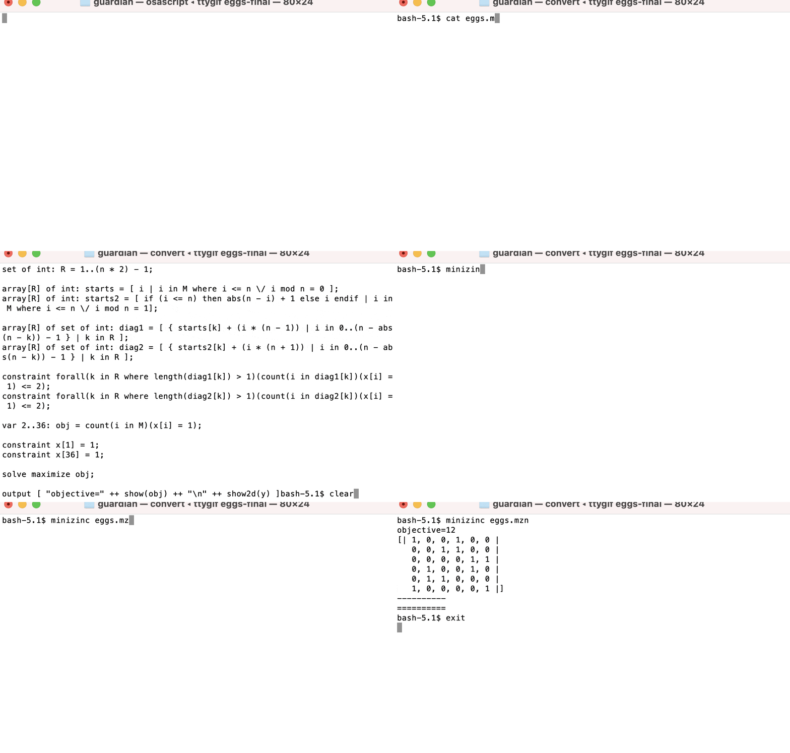
12 again. So even with all those extra restrictions, it is possible to place 12 eggs.
Interestingly if we look at the output our answer doesn’t match Alex’s one.
We’ve found one optimal solution to the problem that places 12 eggs but how many others are there? Well, we can just ask the solver to produce them all!
We need to make a small adjustment to our model to fix the objective to the optimal value and change the definition to be a satisfaction problem. We can then enumerate all the satisfying solutions.
constraint objective = 12;
solve satisfy;
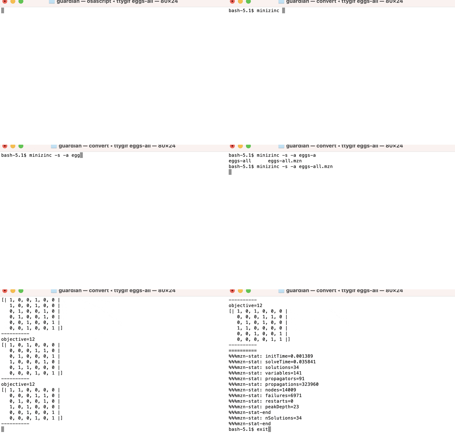
What we see is there are actually 33 other valid placements of 12 eggs.
What have we achieved? Perhaps it’s better to think about what we haven’t done.
We haven’t given any guidance on how to go about solving this problem. We haven’t even defined which solver to run our model against. By default, we’re using Gecode, but we could use exactly the same model with any supported library by only changing the command line argument to:
minizinc --solver coin-bc eggs.mzn or minizinc --solver chuffed eggs.mzn
What we have done is create a concise declarative model of a question we wanted to be answered and we’ve delegated the responsibility to the underlying solver.
We’ve also changed the question we wanted to be answered from finding the maximum number of eggs to finding all the solutions, and again we’ve not had to alter anything other than the model.
For clarity, in the examples, we use fixed dimensions (e.g., 1..36, 1..6, etc.) but we can generalise our model, so we can change it even further without any rework. What if we wanted to find the maximum number of eggs you could place in a 7 by 7 grid such that no dimension has more than 3 eggs on it?

The optimal solution is 21 (when we’ve fixed values in the extreme corners).
Unlike a model produced via some form of Machine Learning, we don’t need any training phase before we can use it. Also, we can make amendments without invalidating earlier computational effort. This particular problem is small enough that we don’t need to invest any time in optimising our search strategy. For larger decision problems this becomes more important.
So what have we learned?
Programming is for the most part imperative; you as the programmer need to be able to instruct (often in tedious detail) how to solve a particular problem. Constraint Programming breaks that dependency. You focus on describing the problem and the computer does the rest.
If you too appreciate the beauty (and fun) of solving decision problems, then we'd like to hear from you. Check out our open roles and join our team at the fastest growing tech company in Scotland.
All source models can be found here.
Get the latest insights and updates delivered to your inbox weekly.
Explore our latest insights and strategies for success.
Discover how AI can transform your resource management and enhance your project delivery.

Get in touch and learn first-hand how Dayshape can help boost profitability, improve client service, and keep your teams happy.
